Abstract: This post will introduce two ways of classify an object using the OpenCV library. It is very good for beginner to study this post because after this you will get an idea of what the whole processing looks like.

Notice: This project was done as the final project for a Computer Vision class at WPI with team member Aditya, Renato and Joe.

As my old habit, let's see this video in order to give you an idea of the results.

Project Problem Statement

In this project, we are given five pink planner objects and we are asked to recognize them with a complex background.

Please pay attention in the computer vision domain about these words: "detect", "recognize", "classify". They have different level of knowing the query objects.

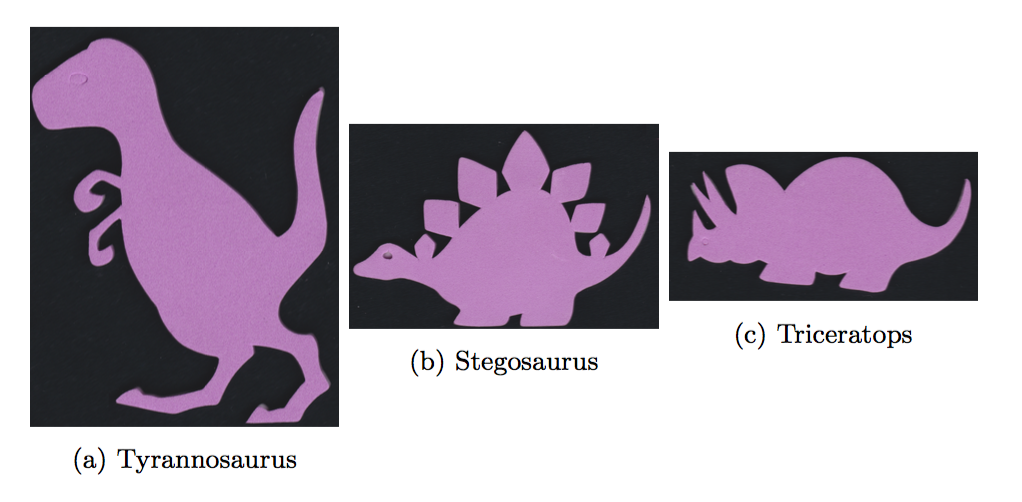
Three of the objects are distinct dinosaurs shown above.

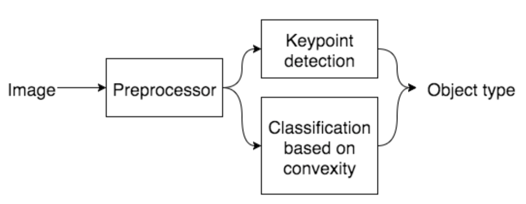
The data flow chart is given. We implemented two methods to finish the task. Notice that each method can do the job, it was just because we want try more, so two.

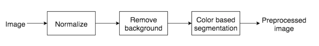
Pre-Processing

It is very crucial to do pre-processing with a query image. Most the cool image stuff we've seen are "draw-back" magic, which mean that layer up the results on the original image instead drawing things directly on it. We will talk about this later on.

Segmentation

Color based segmentation is the process of selecting desired areas of the image based on the color represented. As the image contains noise, the perceived color on each pixel may be distorted, so instead of having a single point on color space, it is more desired to have a range of colors that is accepted.

To better represent the desired range, the color space was converted from BGR (Blue, Green, Red) to HSV (Hue, Saturation, Value). On the converted image, a threshold is applied such that a mask is created to discard every pixel that is not within the determined range.

It is clear that we sample the HSV range from our object first which only designed for the project.

class ColorSegmenter:
    lower_magenta = np.array([125,30,30])
    upper_magenta = np.array([160,255,255])

    @staticmethod
    def getMagentaBlob(bgrimg):
        hsvimg = cv2.cvtColor(bgrimg,cv2.COLOR_BGR2HSV)
        blur = cv2.GaussianBlur(hsvimg,(7,7),0)
        # Threshold the HSV image to get only magenta
        mask = cv2.inRange(blur, ColorSegmenter.lower_magenta, ColorSegmenter.upper_magenta)
        mask = cv2.erode(mask,np.ones((1,1),np.uint8),iterations = 5)
        # mask = cv2.dilate(mask,np.ones((3,3),np.uint8),iterations = 3)
        mask = cv2.morphologyEx(mask,cv2.MORPH_OPEN,np.ones((4,4),np.uint8))
        mask = cv2.morphologyEx(mask,cv2.MORPH_CLOSE,np.ones((15,15),np.uint8))
        # Bitwise-AND mask and original image
        res = cv2.bitwise_and(bgrimg,bgrimg, mask= mask)
        return res

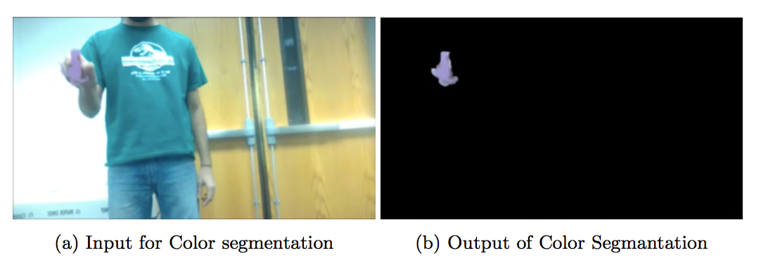
The result of color segmenting is shown above.

Classification based on features

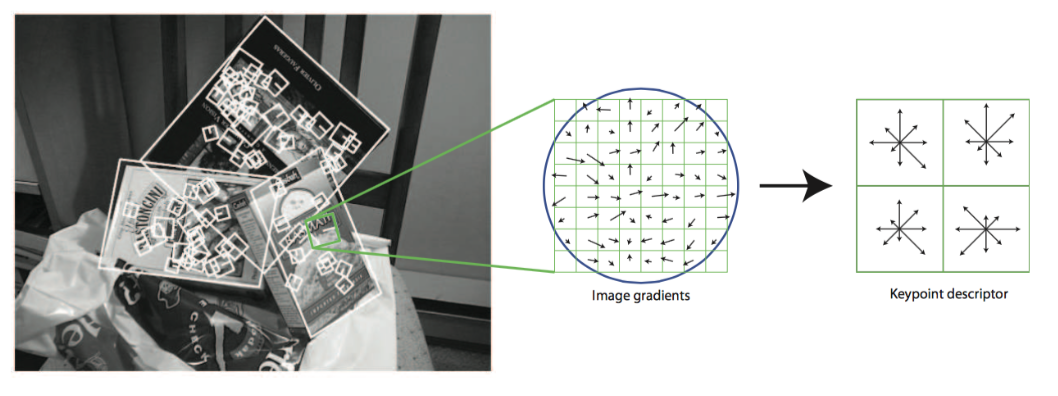
The Key Features could be understood by finding a descriptor in a small part of the image. This descriptor is composited by a lot vectors. Each vector represents some "degree of changing" in the image. For example, the gradient.

The reason why we use this is because Key Features are scale-invariant as well as rotation-invariant. These are the common problem you have to deal with when try to detect something in an image.

In this project, we decide to choose two feature description methods: BRISK and AKAZE. This is due to our queries are planner objects which is lacking of 3D features on the object. These two methods are good at creating descriptors on a binary image or gray scale image. We will briefly talk about how they work.

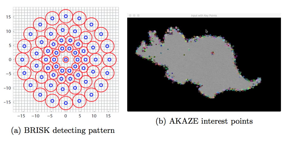
The BRISK use a pattern to calculate the image intensity around a key- point’s neighborhood. The red circle in Figure8a indicates the size of smoothing kernel. It use brightness and pixel orientation to create feature descriptor on a binary image.

The A-KAZE is short for accelerated KAZE feature. It is good for creating feature vectors in a nonlinear scale space. According to the paper[4], they use AOS and variable conductance di↵usion to build a maximum evolution time nonlinear scale space. Then exhibiting a maxima of the Hessian response through the nonlinear scale space, 2D features will be detected. Finally, the main orientation and rotation invariant descriptor in computed by first order derivatives of the 2D features. We apply the AKAZE feature vector generating method on our sample object, as shown above.

def describe(self, image):
    # descriptor = cv2.BRISK_create() #we can use BRISK as well
    descriptor = cv2.AKAZE_create() #we can use BRISK as well

    if self.useSIFT:
        descriptor = cv2.xfeatures2d.SIFT_create()
    # make it gray scaled for 2D features
    self.gray = cv2.cvtColor(image, cv2.COLOR_BGR2GRAY)
    (self.kps, descs) = descriptor.detectAndCompute(self.gray, None)
    #only take the (x,y) attribute and form a NP array.
    kps = np.float32([kp.pt for kp in self.kps]) 

    return (kps, descs)

Sample Database

We use a ”smart” way to store our samples in a .csv file as the database. Once the program is initiated, it will read the .csv file and retrieve sample image paths along with a given sample ID name. After having these information, the program call our feature describing methods to create feature vectors on the samples and same them in the memory for next use.
By writing code this way, we can easily modify our sample database without a line changed in the code.

ap = argparse.ArgumentParser()
ap.add_argument("-d", "--db", required = True, help = "path to the object information database csv file")
ap.add_argument("-s", "--samples", required = True, help = "path to the sample(training) data folder")
ap.add_argument("-q", "--query", required = True, help = "path to the query image")
ap.add_argument("-f", "--sift", type = int, default = 0, help = "use SIFT = 1, not use = 0")

args = vars(ap.parse_args())

db = {}

for line in csv.reader(open(args["db"])):
    db[line[0]] = line[1:]

Matching Queries

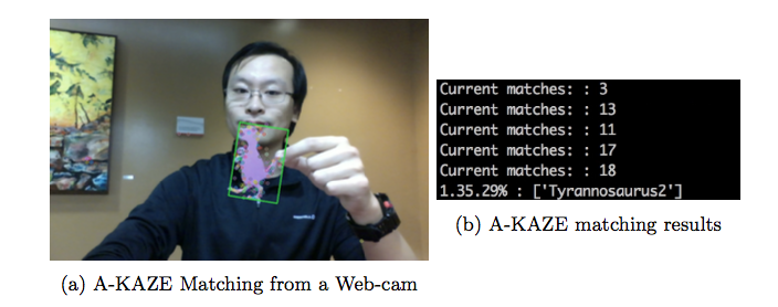
When all the steps above are done, we can finally recognize our query image by comparing our samples to it(notice the comparing direction). A K-NN network is applied here based on a method that can measure the distance between two images which is called ”BruteForce-Hamming” method.

# now match the query obj (B) with our samplebase (A)
def match(self, kpsA, featuresA, kpsB, featuresB):
    matcher = cv2.DescriptorMatcher_create(self.distanceMethod)
    rawMatches = matcher.knnMatch(featuresB, featuresA, 2)
    matches = []

    for m in rawMatches:
        if len(m) == 2 and m[0].distance < m[1].distance * self.ratio:
            #be careful with the train/query orders
            matches.append((m[0].trainIdx, m[0].queryIdx)) 

Notice that, in this project, we are classifying the query to its corresponding sample, so the neighbor number argument we give to KNN is only ’2’; besides this, we apply a 0.7 ratio on the distance to make sure that we get a better result. However, due to the problem that these planner sample image are lacking keypoints in their center area. A high ratio like 0.7 is not always returning a accurate match.

print("{}: {}".format("Current matches: ", len(matches)))

if len(matches) > self.minMatches:
    ptsA = np.float32([kpsA[i] for (i, _) in matches])
    ptsB = np.float32([kpsB[j] for (_, j) in matches])
    (_, status) = cv2.findHomography(ptsA, ptsB, cv2.RANSAC, 4.0)
    # matching ratio against the object in samplebase
    return float(status.sum()) / status.size 

return -1.0 # no possible match

Draw back the results

Now supposing we already have some good matches, the last thing we need to do is find the transformation between two matched keypoints which are in the query image and our sample image. We need at least four matched pairs to do this. The openCV has done this for us, just call the function shown in the code with a finding method RANSAC will give us the answer.

def drawGreenBox(self, queryImage, segImage, kpImage):
    # green box
    gray = cv2.cvtColor(segImage,cv2.COLOR_BGR2GRAY)
    ret,thresh = cv2.threshold(gray,127,255,0)
    (_, cnts, _) = cv2.findContours(thresh,
                                    cv2.RETR_EXTERNAL,
                                    cv2.CHAIN_APPROX_SIMPLE)
    if len(cnts) > 0:
        cnt = sorted(cnts, key = cv2.contourArea, reverse = True)[0]

        rect = np.int32(cv2.boxPoints(cv2.minAreaRect(cnt)))
        cv2.drawContours(kpImage, [rect], -1, (0,255,0),2)

    return kpImage

Now you know a whole progress of an OpenCV classification project but there are still more details not included in this post. You should learn them in the feature.

The repo for this project can be found here.